The goal of this document is to provide a basic structure to use Support Vector Machine (SVM) algorithms to Luminex multi-plex data using the xMAP system. This r markdown document is designed to be scalable and the only requirement is the data is clean and has a category column for training. The data is then divided into training and testing. Once the SVM is trained it can be applied to the testing data set to obtain basic performance statistics and the confusion matrix. If the standard SVMlinear kernel is acceptable, the trained model can be saved and used to predict new samples. This is meant to be a very basic example and the data may not be realistic.
Document summary:
Basic SVM Modeling in R for use with Luminex data
Written by: Eric W. Olle
For use with Luminex generated data
CC-BY-SA license (For the RMD document)
No warranty provided.
Created: Febuary 2022
Edited: Aug. 14, 2022
GitHub Repository for the R-markdown document and the data. The Rmd document text may differ slightly from the blog.
NOTE: Uploaded using knitr and RWordPress packages.
Loading Packages
The following document is meant to be a basic overview of how to use SVM to categorize two or more different groups (i.e. Normal v disease) or different sub-types of similar disease based upon a standard Luminex 10-plex panel This can be applied to larger size panels and different data sets. This is just meant to be an very basic “off the shelf” solution for a standard problem. There are several excellent online resources such as Data Camp as well as some excellent books dedicated to machine learning. The basic references used for this were were: Recognition in Machine Learning by Christopher M. Bishop (2006) and Mastering Machine Learning with R by Cory Lesmeister along with the R package manuals. For additional information on the R code the appropriate package manuals and vignettes were used.
library(tidyverse)  #Easiest best is to do them individually
library(kernlab) # Required for easier repeats and confusion matrix
library(caret)  # This package makes data set splitting easier
More information on tidyverse, kernlab or caret just click the name and a new window will open with the CRAN or package specific website.
Loading data
In this part the data is loaded from a: csv, excel or RDS file For the purpose of teaching a “manufactured” data set was created to be similar to a standard human 10-plex assay. The data is not meant to be realistic and is used for teaching purposes only. This generated data has two categories of samples: Control and a “made up” auto immune disease (AID).
In general there are three steps. First, the data is loaded from an appropriate format. Second, any values that are not appropriate (i.e. a negative number for cytokines concentration) are replaced by an NA. Third, a clean data set is created by removing any rows with NA values which can skew the results. Once clean the data set can be visualized and then divided into training and testing sub-groups for Support Vector Machine Analysis.
This section will verify the data set loaded with checking the first 6 records. If you notice there are records with negative values and this data needs to be cleaned using the tidyverse::dplyr package.
#NOTE:  The file type can also be excel or csv just requires a different read command.

dataset_raw <- readRDS(file = "ml_dataset_raw")

# The following is for other types of files.  Will need to uncomment and correctly configure.
#-----------------------------------------------------------------------------#
# For CSV In rstudio use the import data set verify and copy the command.

# data set_raw <- read.csv(<file>, header = TRUE, sep = ",", quote = "\"", dec = ".")

# For excel files (xls and xlsx)
#library(readxl)
#read_excel(<path>)
#-----------------------------------------------------------------------------#

head(dataset_raw)
## # A tibble: 6 × 11
##   GM_CSF IFN_g IL_1b  IL_2  IL_4  IL_5  IL_6  IL_8 IL_10  TNF_a category
##    <dbl> <dbl> <dbl> <dbl> <dbl> <dbl> <dbl> <dbl> <dbl>  <dbl> <chr>
## 1   63.1  9.02  6.93  24.7  3.96  42.7  302.  52.3 55.6  295.   control
## 2   58.9  7.04  8.55  34.5  3.96  61.6  223.  71.2  8.64 128.   control
## 3   56.2 13.6   6.80  24.4  4.80  50.4  120.  65.2 47.7  -54.1  control
## 4   46.9  8.83  7.86  35.9  3.00  42.4  298.  68.7 38.9  114.   control
## 5   40.2  9.70  8.47  18.9  3.12  72.9  103.  25.9 25.4    7.30 control
## 6   52.2 11.1   6.26  40.5  3.98  56.7  153.  68.4 26.0  127.   control
The above data shows that the data contains some negative numbers and that the category column is not a factor. These will be corrected in the following sections. Please note that the column names use and underscore instead of a dash and have had any special characters (i.e. gamma) removed. This just makes future referencing easier. To see negative numbers check in the TNF_a column.
dataset_raw <- dataset_raw %>%
    replace(., dataset_raw  < 0, NA)

# Looking at the number of rows in the data set prior to NA removal

                                        # filtering out NA


svm_dataset <- dataset_raw %>%
    na.exclude()

# Looking at percent remaining

head(svm_dataset)
## # A tibble: 6 × 11
##   GM_CSF IFN_g IL_1b  IL_2  IL_4  IL_5  IL_6  IL_8 IL_10  TNF_a category
##    <dbl> <dbl> <dbl> <dbl> <dbl> <dbl> <dbl> <dbl> <dbl>  <dbl> <chr>
## 1   63.1  9.02  6.93  24.7  3.96  42.7 302.   52.3 55.6  295.   control
## 2   58.9  7.04  8.55  34.5  3.96  61.6 223.   71.2  8.64 128.   control
## 3   46.9  8.83  7.86  35.9  3.00  42.4 298.   68.7 38.9  114.   control
## 4   40.2  9.70  8.47  18.9  3.12  72.9 103.   25.9 25.4    7.30 control
## 5   52.2 11.1   6.26  40.5  3.98  56.7 153.   68.4 26.0  127.   control
## 6   56.4 11.4   7.44  10.1  2.62  83.7  17.3  54.1  7.08 225.   control
The above data set has had the negative numbers converted to NA’s. This can be any value that is not appropriate for analysis. The data set then is converted to the SVM data set for training and testing by removing the NA’s that may affect the algorithm. The SVM data set has 76.5% of the raw data set.
Concluding thoughts for data set cleaning. A clean data set is required to train any machine learning or AI models. However, be careful on “over cleaning” to fit potential individual/group conditional biases. Do just enough to clean the set such as removing missing values and with VERY large data sets consider removing outliers. Be very careful on using outlier removal if the data set does not have normal distribution or if is a small N-size.
Once the data is cleaned/“tidy data” one column need to be converted to a factor. In this example there are two categories: control and AID (Auto Immune Disease). Remember this is “fake” data so these can be called any name.
svm_dataset$category <- as.factor(svm_dataset$category)

head(svm_dataset)
## # A tibble: 6 × 11
##   GM_CSF IFN_g IL_1b  IL_2  IL_4  IL_5  IL_6  IL_8 IL_10  TNF_a category
##    <dbl> <dbl> <dbl> <dbl> <dbl> <dbl> <dbl> <dbl> <dbl>  <dbl> <fct>
## 1   63.1  9.02  6.93  24.7  3.96  42.7 302.   52.3 55.6  295.   control
## 2   58.9  7.04  8.55  34.5  3.96  61.6 223.   71.2  8.64 128.   control
## 3   46.9  8.83  7.86  35.9  3.00  42.4 298.   68.7 38.9  114.   control
## 4   40.2  9.70  8.47  18.9  3.12  72.9 103.   25.9 25.4    7.30 control
## 5   52.2 11.1   6.26  40.5  3.98  56.7 153.   68.4 26.0  127.   control
## 6   56.4 11.4   7.44  10.1  2.62  83.7  17.3  54.1  7.08 225.   control
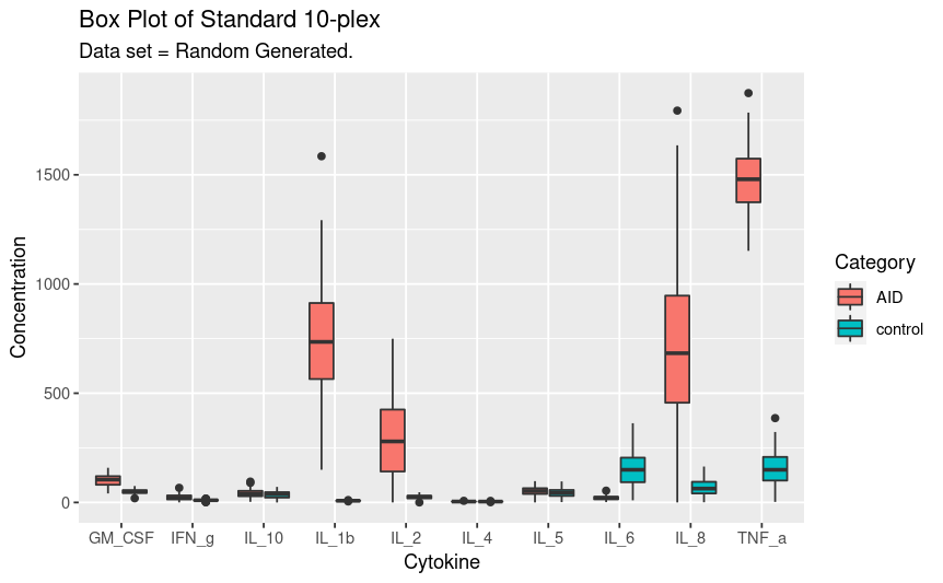
The next step is to perform a basic visual inspection of the data. This is using a box plot to show overall distribution and outliers. Remember this is a data set generated using the random normal variable so there may appear to be “outliers” but this is just part of the model.
# Need to gather the data from column format to a long format for use
# with ggplot.  This is why the gather() is used with the SVM data
# set.

ggplot(gather(svm_dataset,
               key = "Analyte" ,
               value = "Concentration",
              1:10), aes(x = factor(Analyte),
                         y = Concentration,
                         fill = category)) +
    geom_boxplot() +
    labs(title = "Box Plot of Standard 10-plex",
         subtitle = "Data set = Random Generated.",
         fill = "Category") +
    xlab("Cytokine") +
    ylab("Concentration")
Creating the SVM model
First divide into training and testing data. THIS IS ABSOLUTELY REQUIRED. Using the same data to train and test can lead to over-fitting and/or over estimating the models fit. See the caret package for more information on dividing into training and validation sets.
# NOTE: using the caret package to make this easier.
# NOTE:  p value can be changed between 0.6 and 0.8 at user discretion.

training <- caret::createDataPartition(y = svm_dataset$category,
                                       p = 0.70,
                                       list = FALSE)


svm_training <- svm_dataset[ training,]
svm_testing  <- svm_dataset[-training,]
Next step is to do a very basic SVM model with a linear kernel This is using KernLab and allows for easier repeats using training control. See the KernLab package for more information. In this example 10-fold with three repeat cross-validation is performed.
trnctrl <- trainControl(method = "repeatedcv", number = 10, repeats = 3)

svm  <- train(category ~., data = svm_training, method = "svmLinear",
                    trControl = trnctrl,
                    preProcess =  c("center", "scale"),
                    tuneLength = 10)
print(svm)
## Support Vector Machines with Linear Kernel
##
## 215 samples
##  10 predictor
##   2 classes: 'AID', 'control'
##
## Pre-processing: centered (10), scaled (10)
## Resampling: Cross-Validated (10 fold, repeated 3 times)
## Summary of sample sizes: 193, 193, 194, 193, 193, 193, ...
## Resampling results:
##
##   Accuracy  Kappa
##   1         1
##
## Tuning parameter 'C' was held constant at a value of 1
The above shows how the SVM was trained. The next step is to test it against the testing partition.
svm_pred <- predict(svm , svm_testing)

## Other plus of using kernlab is the easier confusion matrix generation

confusionMatrix(table(svm_pred, svm_testing$category))
## Confusion Matrix and Statistics
##
##
## svm_pred  AID control
##   AID      41       0
##   control   0      50
##
##                Accuracy : 1
##                  95% CI : (0.9603, 1)
##     No Information Rate : 0.5495
##     P-Value [Acc > NIR] : < 2.2e-16
##
##                   Kappa : 1
##
##  Mcnemar's Test P-Value : NA
##
##             Sensitivity : 1.0000
##             Specificity : 1.0000
##          Pos Pred Value : 1.0000
##          Neg Pred Value : 1.0000
##              Prevalence : 0.4505
##          Detection Rate : 0.4505
##    Detection Prevalence : 0.4505
##       Balanced Accuracy : 1.0000
##
##        'Positive' Class : AID
##
The confusion matrix and the statistics shows how the model performs. This was a simple model but in more complex models, missed calls are common and will be show in the confusion matrix and SVM statistics.
Using the SVM model to predict the category
In real world scenarios, the SVM model would be saved, and this next section would be a separate r markdown document (or r script) that would be used just for prediction. For ease of teaching the predicting was show as part of the same r markdown file.
Using a new data set created with another random generation seed. This data set has the same underlying distributions of the original data but was created separately. This set kept the category but will be “blinded” and then tested. The data was cleaned prior to saving to make this section easier. The data is blinded (i.e. category removed) prior to adding the SVM prediction column. This column could be kept and a secondary confusion matrix generated using data never seen by the initial model.
#loading the data set
new_data <- readRDS("ml_predict_set")
#blinding the data
blind_new_data <- select(new_data, -category)
#predicting the category
new_data_predict <- predict(svm,  blind_new_data)

# column binding the new data predictions

full_new_data <- cbind(blind_new_data, Prediction = new_data_predict)

## Looking at the full table

knitr::kable(full_new_data, digits = 2)
| GM_CSF | IFN_g | IL_1b | IL_2 | IL_4 | IL_5 | IL_6 | IL_8 | IL_10 | TNF_a | Prediction |
|---|---|---|---|---|---|---|---|---|---|---|
| 45.15 | 10.73 | 9.64 | 27.26 | 4.63 | 22.77 | 103.30 | 5.41 | 32.28 | 150.85 | control |
| 56.76 | 9.60 | 7.86 | 20.98 | 3.06 | 48.04 | 153.07 | 49.66 | 45.54 | 199.97 | control |
| 39.00 | 14.66 | 11.63 | 14.93 | 3.79 | 68.88 | 185.20 | 108.02 | 67.67 | 175.95 | control |
| 48.61 | 13.06 | 8.58 | 34.99 | 4.79 | 20.66 | 164.18 | 103.51 | 33.07 | 231.79 | control |
| 90.66 | 9.54 | 376.32 | 168.62 | 3.87 | 49.44 | 6.69 | 1253.82 | 55.31 | 1480.62 | AID |
| 47.68 | 10.04 | 9.70 | 41.41 | 2.60 | 83.00 | 144.63 | 102.30 | 21.07 | 226.53 | control |
| 47.02 | 22.77 | 826.63 | 540.84 | 6.00 | 23.17 | 18.70 | 735.88 | 36.29 | 1525.37 | AID |
| 59.06 | 6.88 | 7.32 | 15.64 | 4.19 | 41.25 | 170.61 | 9.66 | 48.63 | 212.37 | control |
| 49.69 | 7.86 | 5.74 | 12.84 | 5.65 | 30.43 | 32.91 | 127.76 | 42.81 | 236.62 | control |
| 120.93 | 26.57 | 744.32 | 515.47 | 3.15 | 55.91 | 28.72 | 665.02 | 10.23 | 1315.09 | AID |
| 77.11 | 17.22 | 1060.71 | 193.29 | 2.70 | 68.65 | 16.02 | 807.98 | 18.45 | 1412.12 | AID |
| 117.26 | 14.24 | 476.25 | 192.52 | 5.07 | 64.48 | 22.67 | 1055.61 | 23.72 | 1546.70 | AID |
| 93.12 | 2.58 | 149.57 | 133.90 | 2.40 | 54.45 | 31.86 | 264.05 | 37.49 | 1468.69 | AID |
| 44.18 | 7.64 | 8.92 | 30.49 | 4.54 | 30.89 | 201.93 | 86.71 | 39.14 | 81.04 | control |
| 55.81 | 8.61 | 7.75 | 14.10 | 3.54 | 35.54 | 273.52 | 105.32 | 44.53 | 106.76 | control |
| 107.48 | 6.24 | 775.88 | 287.56 | 4.29 | 36.06 | 26.60 | 867.58 | 23.80 | 1708.22 | AID |
| 85.42 | 20.05 | 1083.64 | 507.51 | 4.65 | 53.44 | 19.93 | 245.13 | 67.78 | 1678.81 | AID |
| 123.01 | 24.84 | 658.85 | 287.20 | 4.22 | 2.64 | 9.86 | 613.03 | 58.70 | 1571.94 | AID |
| 44.82 | 38.64 | 515.85 | 373.81 | 4.26 | 37.58 | 7.40 | 134.69 | 11.72 | 1943.04 | AID |
| 50.69 | 12.30 | 8.49 | 23.97 | 3.15 | 48.20 | 119.94 | 132.93 | 23.66 | 204.96 | control |
| 104.38 | 1.03 | 567.50 | 259.82 | 3.80 | 67.48 | 26.97 | 908.13 | 64.89 | 1686.21 | AID |
| 77.82 | 9.49 | 770.94 | 152.51 | 2.66 | 48.31 | 18.15 | 1032.94 | 54.89 | 1496.37 | AID |
| 42.06 | 9.07 | 6.42 | 20.12 | 3.32 | 16.04 | 140.56 | 125.10 | 47.20 | 225.16 | control |
| 52.35 | 8.96 | 6.36 | 17.99 | 3.24 | 25.95 | 188.72 | 18.97 | 17.48 | 137.01 | control |
| 39.78 | 11.65 | 8.18 | 27.06 | 3.81 | 53.80 | 211.01 | 99.86 | 31.68 | 186.67 | control |
| 86.75 | 24.53 | 1459.89 | 318.42 | 4.88 | 59.93 | 29.95 | 339.68 | 22.43 | 1663.64 | AID |
| 45.44 | 9.61 | 8.13 | 25.72 | 3.60 | 43.93 | 107.71 | 95.43 | 11.14 | 233.01 | control |
| 61.25 | 9.59 | 5.93 | 37.21 | 3.74 | 47.34 | 25.09 | 41.54 | 55.82 | 144.40 | control |
| 49.36 | 10.41 | 7.49 | 12.87 | 2.78 | 5.14 | 113.20 | 53.77 | 15.59 | 155.97 | control |
| 80.88 | 18.11 | 712.40 | 25.41 | 4.28 | 43.92 | 13.54 | 788.88 | 61.19 | 1486.55 | AID |
| 38.36 | 6.89 | 6.93 | 16.18 | 2.81 | 43.97 | 38.02 | 104.68 | 24.34 | 283.90 | control |
| 46.78 | 7.09 | 8.80 | 25.47 | 3.94 | 47.31 | 273.56 | 65.29 | 36.03 | 96.89 | control |
| 93.62 | 19.72 | 539.32 | 126.67 | 4.64 | 54.85 | 16.15 | 850.38 | 18.50 | 1552.92 | AID |
| 100.72 | 5.36 | 1586.33 | 481.88 | 4.36 | 49.57 | 4.42 | 526.38 | 31.77 | 1482.74 | AID |
| 52.84 | 22.02 | 376.19 | 131.67 | 2.64 | 25.64 | 35.09 | 604.77 | 31.96 | 1445.43 | AID |
| 39.43 | 10.92 | 5.74 | 16.90 | 4.32 | 66.06 | 86.62 | 54.89 | 56.16 | 142.36 | control |
| 46.31 | 10.29 | 8.11 | 13.88 | 3.57 | 50.75 | 281.64 | 92.47 | 36.92 | 241.68 | control |
| 102.07 | 24.93 | 893.10 | 558.56 | 2.13 | 49.80 | 34.97 | 1617.69 | 30.42 | 1393.30 | AID |
| 83.78 | 40.86 | 825.13 | 130.94 | 3.27 | 62.37 | 22.84 | 941.08 | 28.59 | 1554.44 | AID |
| 34.85 | 10.69 | 7.40 | 20.33 | 3.97 | 34.92 | 40.37 | 90.17 | 14.86 | 129.51 | control |
| 42.97 | 12.69 | 6.42 | 36.56 | 2.83 | 60.02 | 224.31 | 155.31 | 12.39 | 171.33 | control |
| 73.12 | 25.33 | 835.94 | 308.63 | 4.00 | 63.71 | 39.73 | 1408.66 | 25.67 | 1614.76 | AID |
| 39.53 | 13.15 | 7.59 | 33.78 | 3.31 | 12.61 | 185.66 | 63.87 | 28.72 | 208.48 | control |
| 129.87 | 29.52 | 1334.98 | 140.73 | 2.47 | 30.68 | 29.22 | 573.86 | 31.18 | 1604.78 | AID |
| 45.85 | 11.57 | 7.68 | 28.60 | 4.57 | 13.68 | 87.83 | 94.26 | 9.48 | 154.67 | control |
| 107.39 | 48.65 | 779.78 | 394.60 | 1.70 | 92.83 | 22.86 | 1192.12 | 25.88 | 1524.06 | AID |
| 74.77 | 41.76 | 801.34 | 110.19 | 4.80 | 55.02 | 33.84 | 414.64 | 80.28 | 1633.50 | AID |
| 65.93 | 15.20 | 10.21 | 24.39 | 3.78 | 46.39 | 186.77 | 137.14 | 27.69 | 50.78 | control |
| 75.21 | 24.53 | 446.47 | 125.66 | 2.34 | 42.10 | 14.89 | 327.23 | 50.97 | 1579.51 | AID |
| 45.86 | 6.01 | 6.70 | 23.67 | 4.07 | 20.28 | 50.54 | 64.46 | 25.64 | 161.60 | control |
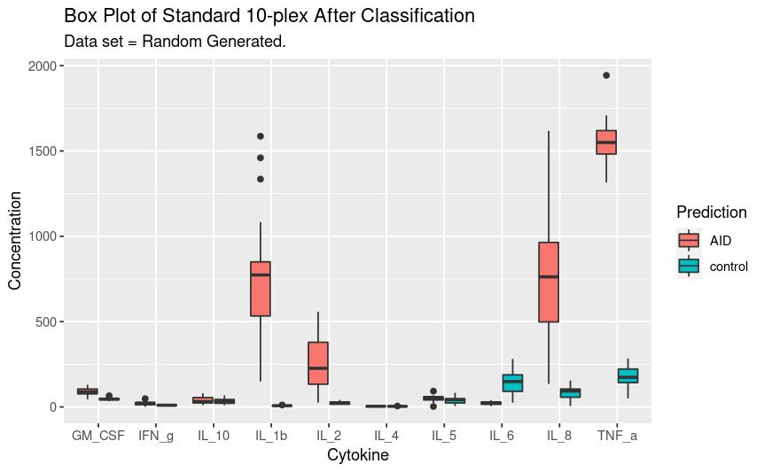
The above table shows the prediction attached to the data. The data was blinded this experiment can be repeated without removing the classifier and a confusion matrix generated to determine model efficacy.
Finally, the full new data set with predictions can be plotted as above.
## Visualizing the predicted new data

ggplot(gather(full_new_data,
               key = "Analyte" ,
               value = "Concentration",
              1:10), aes(x = factor(Analyte),
                         y = Concentration,
                         fill = Prediction)) +
    geom_boxplot() +
    labs(title = "Box Plot of Standard 10-plex After Classification",
         subtitle = "Data set = Random Generated.",
         fill = "Prediction") +
    xlab("Cytokine") +
    ylab("Concentration")
SVM is a robust method for classification and can easily be applied to cytokine multiplex data generated using instruments like the Luminex Bead Based Array system.