Part 2: Generating a layered pseudo-3D map using R
The goal of this document is to modify and use a rotate_sf() function written by Stephan Junger and Denis Cohen in the “Method Bytes” blog. The function was modified to allow the user to change the shear matrix and the angle of rotation (theta). Additionally, the rotation calculation was slightly modified to approximate the theta requested by the user. This is meant to modify an excellent function written by Junger and Cohen and will be added at a later date to another package (trauma directors tool kit tdtk).
This is the second part of a three-part series on basic geo-spatial in R using census data. In part one census data was plotted for different variables and then graphed. Part two looks at rotating and separating the layers in a pseudo 3D projection. Finally, in part 3 a bivariate color scheme will be used a generated to show how to plot two variable in a low, moderate and high categories. Census data was chosen since it is easy to find basic statistics that are matched to the necessary geometry files. A lot of the work is derived from existing references such as: TidyCensus, CensusAPI and blog posts.
Why is it important to use a rotated projection? In geo-spatial analysis it is easy to get overwhelmed by multiple variables that can be projected in separate plots (Part 1: Basic geo-spatial using R) or as a bivariate color scheme. In this basic but not optimal example, the number of individuals at different level of the poverty line were extracted and displayed. This was done using the tidycensus package to interface with the 2020 5 year-American Community Survey data. This data contains different subsets of the poverty line (i.e. < 0.5, 0.5 to < 1.0 and 1.0 to < 1.5 – times the poverty line) and does not fit into a standard bi or tri-variate color scheme (See Dr. Cynthia Brewers work at Penn State Univ). The separation and rotation of the layers allows for a rapid visualization of how the number of individuals at different levels of the poverty line changes on a census tract level.
The basic equation used to convert a 2D to pseudo3D image is as follows:
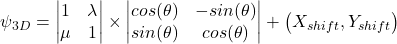
The rotate_sf() uses a shear matrix, a rotation matrix and a shift and coverts the geometry coordinates to a different perspective. The function takes an angle theta in degrees and converts to rad. The shear matrix uses values lambda and mu to shift parallel to the Y or X, axis. Finally, the shift X or shift y adds shift to the spatial frame geometry to offset the values and minimize overlap.
Document summary:
Generating a layered pseudo-3D map using R
Written by: Pete Skach and Eric W. Olle
CC-BY-SA license for the r-markdown document.
GPLv3 for the code.
Make sure you visit the Junger and Cohen blog (reference below).
No Warranty Provided
Created: Oct 2022
Edited for blog: October 14, 2022
The GitHub for this project contains the R-markdown and the data used to generate this blog. The data and the markdown document are CC-BY-SA.
Loading the packages
Once the packages are loaded the next step is to get the US Census Data with the geospatial geometry. Check out the tidycensus package for more information on how to retrieve the data. Make sure you have the your census API token correctly configured or no data will be retrieved.
Getting the Census data
This is using the data from a 5-year American Community Survey but can be a range of different sources including the 10-year full census. For information on the variable list see:
https://api.census.gov/data/2020/acs/acs5/variables.html
WV_poverty <- get_acs(
  state = "WV",
  geography = "tract",
  variables = c(total = "C18131_001E",
                lt05 = "C18131_002E",
                gt5to99 = "C18131_005E",
                gt1to15 = "C18131_008E"),
  geometry = TRUE,
  output = "wide",
  year = 2020)
## Getting data from the 2016-2020 5-year ACS
## Using FIPS code '54' for state 'WV'
names(WV_poverty)
##  [1] "GEOID"       "NAME"        "total"       "C18131_001M" "lt05"
##  [6] "C18131_002M" "gt5to99"     "C18131_005M" "gt1to15"     "C18131_008M"
## [11] "geometry"
Looking at the column names shows that the geometry was loaded along with the data with margin of error. This can be verified with a simple “head()” command. This will also verify that it is a spatial data frame.
head(WV_poverty)
## Simple feature collection with 6 features and 10 fields
## Geometry type: POLYGON
## Dimension:     XY
## Bounding box:  xmin: -82.54137 ymin: 38.39577 xmax: -79.80879 ymax: 40.05918
## Geodetic CRS:  NAD83
##         GEOID                                             NAME total
## 1 54001965700 Census Tract 9657, Barbour County, West Virginia  4932
## 2 54001965500 Census Tract 9655, Barbour County, West Virginia  3845
## 3 54069001300      Census Tract 13, Ohio County, West Virginia  1352
## 4 54011001400    Census Tract 14, Cabell County, West Virginia  2332
## 5 54011001900    Census Tract 19, Cabell County, West Virginia  2405
## 6 54099005100     Census Tract 51, Wayne County, West Virginia  1891
##   C18131_001M lt05 C18131_002M gt5to99 C18131_005M gt1to15 C18131_008M
## 1         506  377         205     355         262     577         258
## 2         457  286         167     530         351     168         118
## 3         258   79          58      79          54      73          54
## 4         474  576         303     421         264     179         104
## 5         305   87          59     207         106     182         132
## 6         183   78          59     288         152     211          89
##                         geometry
## 1 POLYGON ((-80.07606 39.1016...
## 2 POLYGON ((-80.22631 39.1235...
## 3 POLYGON ((-80.72345 40.0347...
## 4 POLYGON ((-82.43736 38.4168...
## 5 POLYGON ((-82.40455 38.4074...
## 6 POLYGON ((-82.54137 38.3963...
Notice that for each of the values there is a Margin of Error indicated by an M at the end of the variable identifier. This is part of the American Community Survey that estimates values from a sample. This is not present in the decennial census. Next is to load a modified rotate_sf() originally developed by Junger and Cohen (see link at the end for the initial version). If the rotate_sf() is not shown due to the collapse = TRUE on Rmd, please check the github for the code.
Looking at a sum of the poverty line data
On way commonly used in geo-spatial analysis is to sum the different groups that meet a specified criteria and then display as a total N, rate or probability. In this next case, the probability of being less than 1.5-times the poverty was calculated. The tidycensus package offers the ability to sum the margin of error using the moe_sum(). This was not done because this was just used as an example and not for direct statistical comparison.
WV_poverty %>%
    rowwise() %>%
    mutate(pvrty_est = sum(c(lt05, gt5to99, gt1to15))) %>%
    mutate(pvrty_ratio = pvrty_est/total) -> WV_poverty_sum


WV_poverty_sum %>%
    ggplot(aes(fill =  pvrty_ratio)) +
    geom_sf(color = "black") +
    theme_void() +
    scale_fill_viridis_c(option = "turbo") +
        theme(plot.title = element_text(hjust = 0.5),
          plot.subtitle = element_text(hjust = 0.5)) +
    labs(title = "Number with a Poverty Ratio (< 0.5 to 1.50) by Census Tract.",
         caption = "2020 ACS data.",
         subtitle = "Sum of N bellow 1.5-times poverty line / total",
         fill = "Probability")

This a a probability based upon the calculated “total” variable from the US Census data. These are summed. This may however not be the best way to summarize the data due to the Margin of Error (MOE) associated with US Census ACS estimates. Additionally, sometimes one or more variables need to be show concurrently but it is not amenable to a faceted or side-by-side display. With a A “flat_state” geo-spatial plot can be expressed as a pseudo-3D object by rotating and separating the layers along with the role of theta, lambda and mu in the rotation and shear matrices.
Pseudo-3D with Basic Junger and Cohen defaults
In this first plot, the basic Junger and Cohen defaults were use to display the poverty line data. In this version of rotate_sf(), the angle in degrees is entered and converted to radians. An eight-degree theta was chosen as default because it is close to the Junger and Cohen pi/20 theta.
ggplot() +
    geom_sf(data = rotate_sf(WV_poverty, theta = 8), fill = "white", color = "black", alpha = 0.1) +
    geom_sf(data = rotate_sf(WV_poverty,theta = 8, y_add = 2, x_add = -0.5), aes(fill = lt05),
            alpha = .5) +
     geom_sf(data = rotate_sf(WV_poverty,theta = 8, y_add = 4, x_add = -0.5), aes(fill = gt5to99),
             alpha = .5) +
    geom_sf(data = rotate_sf(WV_poverty,theta = 8, y_add = 6, x_add = -0.5), aes(fill = gt1to15),
            alpha = .5) +
    scale_fill_viridis_c(option = "turbo") +
    theme_void() +
   labs(title = "Pseudo-3D plot of US Census Data",
         subtitle = "Default shear matrix and a rotation of 8 degrees",
         fill = "N in tract")
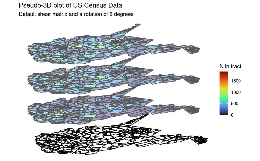
Now that the basic display using the established methods, next it to show the effect of rotation
Modifying the theta (added functionality)
In this example, the theta was changed to show a negative rotation. The plot is rotated to a negative eight degrees.
ggplot() +
    geom_sf(data = rotate_sf(WV_poverty, theta =-8), fill = "white", color = "black", alpha = 0.1) +
    geom_sf(data = rotate_sf(WV_poverty,theta = -8, y_add = 2, x_add = -0.3), aes(fill = lt05),
            alpha = 0.5) +
     geom_sf(data = rotate_sf(WV_poverty,theta = -8, y_add = 4, x_add = -0.5), aes(fill = gt5to99),
             alpha = 0.5) +
    geom_sf(data = rotate_sf(WV_poverty,theta = -8, y_add = 6, x_add = -0.5), aes(fill = gt1to15),
            alpha = 0.5) +
    scale_fill_viridis_c(option = "turbo") +
    theme_void() +
   labs(title = "Pseudo-3D plot of US Census Data",
         subtitle = "Default shear matrix and a rotation of -8 degrees",
         fill = "N in tract")
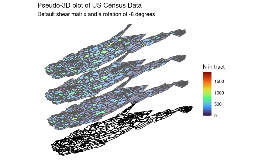
The change in angle of display is clearly shown when you compare figure 2 and 3.
Modifying the Shear matrix
The shear matrix sets the amount the X and Y values are “sheared” parallel to the X or Y axis. From equation shown in the introduction the Junger and Cohen used a shear matrix that does not maintain the area. Additional, the diagonal matrix usually is populated with ones. The next several steps will play with different iterations of lambda and mu along with showing how to maintain the area. Finally, a matrix that “plays around” with the values to obtain decent stacked view.
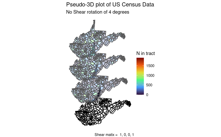
Modifying the shear matrix to 0 lambda and mu
Notice how setting the UR and LL values to 0 “flatten” the data.
new_shear <- c(1, 0, 0, 1)


ggplot() +
    geom_sf(data = rotate_sf(WV_poverty, shear_values = new_shear, theta = 4), fill = "white", color = "black", alpha = 0.1) +
    geom_sf(data = rotate_sf(WV_poverty, shear_values = new_shear, theta =  4, y_add = 2, x_add = -0.3), aes(fill = lt05),
            alpha = 0.3) +
     geom_sf(data = rotate_sf(WV_poverty, shear_values = new_shear, theta =  4, y_add = 4, x_add = -0.5), aes(fill = gt5to99),
             alpha = 0.3) +
    geom_sf(data = rotate_sf(WV_poverty, shear_values = new_shear, theta = 4, y_add = 6, x_add = -0.5), aes(fill = gt1to15),
            alpha = 0.3) +
    scale_fill_viridis_c(option = "turbo") +
    theme_void() +
     labs(title = "Pseudo-3D plot of US Census Data",
         subtitle = "No Shear rotation of 4 degrees",
         caption =  paste("Shear matix = " ,paste(new_shear, collapse = ", ")),
         fill = "N in tract")
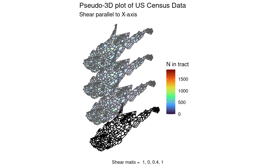
Modifying the lambda only
Adding a positive value to the the lambda variable will shift the values parallel to the X-axis.
new_shear <- c(1, 0, 0.4, 1) # Changing the matrix


ggplot() +
    geom_sf(data = rotate_sf(WV_poverty, shear_values = new_shear, theta = 8), fill = "white", color = "black", alpha = 0.1) +
    geom_sf(data = rotate_sf(WV_poverty, shear_values = new_shear, theta =  8, y_add = 2, x_add = -0.3), aes(fill = lt05),
            alpha = 0.3) +
     geom_sf(data = rotate_sf(WV_poverty, shear_values = new_shear, theta =  8, y_add = 4, x_add = -0.5), aes(fill = gt5to99),
             alpha = 0.3) +
    geom_sf(data = rotate_sf(WV_poverty, shear_values = new_shear, theta = 8, y_add = 6, x_add = -0.5), aes(fill = gt1to15),
            alpha = 0.3) +
    scale_fill_viridis_c(option = "turbo") +
    theme_void()  +
     labs(title = "Pseudo-3D plot of US Census Data",
         subtitle = "Shear parallel to X-axis",
         caption =  paste("Shear matix = " ,paste(new_shear, collapse = ", ")),
         fill = "N in tract")
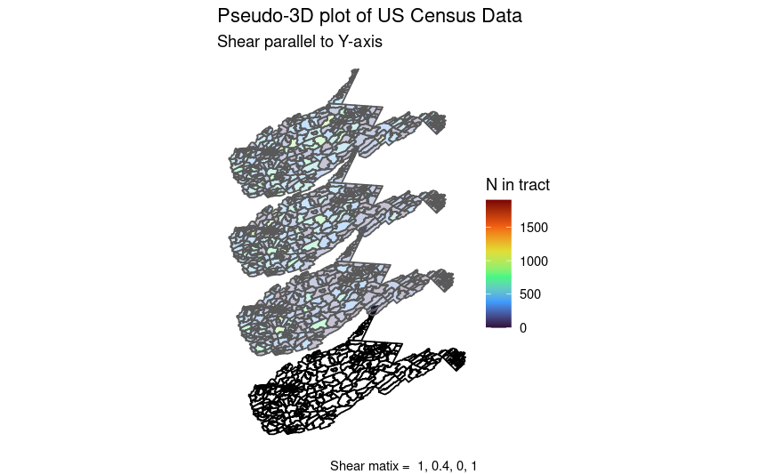
Modifying mu only
This should shift the values parallel to the Y-axis.
new_shear <- c(1, 0.4, 0, 1)


ggplot() +
    geom_sf(data = rotate_sf(WV_poverty, shear_values = new_shear, theta = 4), fill = "white", color = "black", alpha = 0.1) +
    geom_sf(data = rotate_sf(WV_poverty, shear_values = new_shear, theta =  4, y_add = 2, x_add = -0.3), aes(fill = lt05),
            alpha = 0.3) +
     geom_sf(data = rotate_sf(WV_poverty, shear_values = new_shear, theta =  4, y_add = 4, x_add = -0.5), aes(fill = gt5to99),
             alpha = 0.3) +
    geom_sf(data = rotate_sf(WV_poverty, shear_values = new_shear, theta = 4, y_add = 6, x_add = -0.5), aes(fill = gt1to15),
            alpha = 0.3) +
    scale_fill_viridis_c(option = "turbo") +
    theme_void()  +
     labs(title = "Pseudo-3D plot of US Census Data",
         subtitle = "Shear parallel to Y-axis",
         caption =  paste("Shear matix = " ,paste(new_shear, collapse = ", ")),
         fill = "N in tract")
To combine both do a basic composition matrix of [1+(mu*lambda), mu, lambda, 1]. Although a better method maybe to “play around” with the values. One issue with “playing around” with the shear matrix to get the desired projection the plot area may not be preserved.
Modifying shear matrix to maintain equal area
This is done be setting the UL value of the shear matrix to 1 + (lambda * mu)
new_shear <- c(1.08, 0.4, 0.2, 1)


ggplot() +
    geom_sf(data = rotate_sf(WV_poverty, shear_values = new_shear, theta = 4), fill = "white", color = "black", alpha = 0.1) +
    geom_sf(data = rotate_sf(WV_poverty, shear_values = new_shear, theta =  4, y_add = 2, x_add = -0.3), aes(fill = lt05),
            alpha = 0.3) +
     geom_sf(data = rotate_sf(WV_poverty, shear_values = new_shear, theta =  4, y_add = 4, x_add = -0.5), aes(fill = gt5to99),
             alpha = 0.3) +
    geom_sf(data = rotate_sf(WV_poverty, shear_values = new_shear, theta = 4, y_add = 6, x_add = -0.5), aes(fill = gt1to15),
            alpha = 0.3) +
    scale_fill_viridis_c(option = "turbo") +
    theme_void() +
     labs(title = "Pseudo-3D plot of US Census Data",
         subtitle = "Preserving Area in Shear matrix UL = 1+ lambda*mu",
         caption =  paste("Shear matix = " ,paste(new_shear, collapse = ", ")),
         fill = "N in tract")

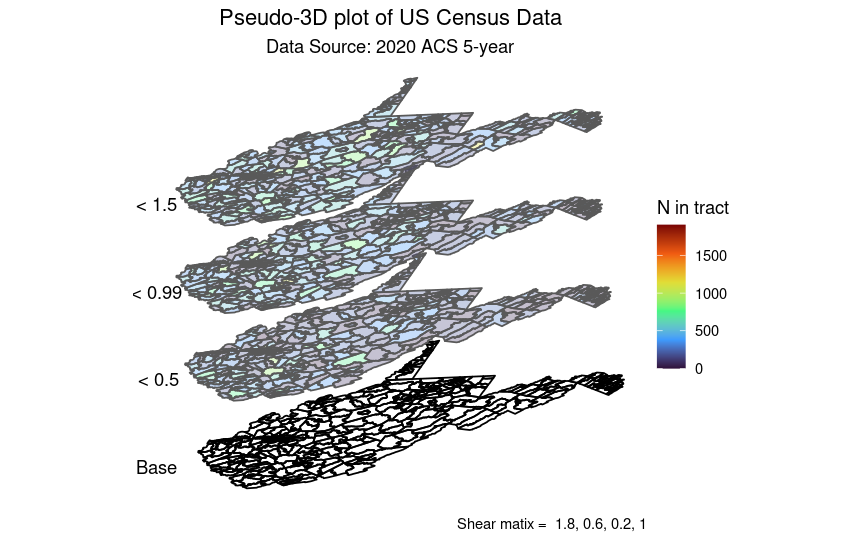
In one of the iterations of a shear matrix the following seemed to work well. It slightly modified the upper left to be 1+(lambda + mu). This may not maintain the area but seemed to provides a good visualization of the state.
Modifying the shear matrix to provide “optimal” views.
new_shear <- c(1.8, 0.6, 0.2, 1)

ggplot() +
    geom_sf(data = rotate_sf(WV_poverty, shear_values = new_shear, theta = 4), fill = "white", color = "black", alpha = 0.1) +
    geom_sf(data = rotate_sf(WV_poverty, shear_values = new_shear, theta =  4, y_add = 2, x_add = -0.3), aes(fill = lt05),
            alpha = 0.3) +
     geom_sf(data = rotate_sf(WV_poverty, shear_values = new_shear, theta =  4, y_add = 4, x_add = -0.5), aes(fill = gt5to99),
             alpha = 0.3) +
    geom_sf(data = rotate_sf(WV_poverty, shear_values = new_shear, theta = 4, y_add = 6, x_add = -0.5), aes(fill = gt1to15),
            alpha = 0.3) +
    scale_fill_viridis_c(option = "turbo") +
    theme_void() +
    theme(plot.title = element_text(hjust = 0.5),
          plot.subtitle = element_text(hjust = 0.5))  +
    annotate("text", x = -125, y = 30, label = "Base") +
    annotate("text", x = -125, y = 32, label = " < 0.5") +
    annotate("text", x = -125, y = 34, label = "< 0.99") +
    annotate("text", x = -125, y = 36, label = "< 1.5") +
    labs(title = "Pseudo-3D plot of US Census Data",
         subtitle = "Data Source: 2020 ACS 5-year",
         caption =  paste("Shear matix = " ,paste(new_shear, collapse = ", ")),
         fill = "N in tract")
Conclusion
The initial rotate_sf() by Junger and Cohen is an excellent function for adding “depth” to a 2D plot. This allows for separation of layer and create an plot that can display multiple values in a “stacked” versus “faceted” method. This version of the rotate_sf() function builds on their excellent work by adding user option to rotate based upon degrees that are later converted to rad. Additionally, this function allows the end user to change the shear matrix and create a plot optimal for the data.
Referenced function (also on referenced github page):
rotate_sf <- function(data,
                      shear_values = c(2, 1.2, 0, 1),
                      theta = 4,
                      x_add = 0,
                      y_add = 0)
{

    shear_matrix <- function (x)
    {
    matrix(shear_values, 2, 2)
  }

    rotate_matrix <- function(x)
    {
    matrix(c(cos(x), sin(x), -sin(x), cos(x)), 2, 2)
  }


    # Due to equal matrix dimensions, standard multipliccation (*) or
    # inner produce (%*%) will work (see below where inner product is
    # used)
  data %>%
    dplyr::mutate(
      geometry =
        .$geometry * shear_matrix() %*% rotate_matrix((pi/180) * theta) + c(x_add, y_add)
    )
}
Session information
## R version 4.2.1 (2022-06-23)
## Platform: x86_64-pc-linux-gnu (64-bit)
## Running under: Pop!_OS 20.04 LTS
##
## Matrix products: default
## BLAS:   /usr/lib/x86_64-linux-gnu/openblas-pthread/libblas.so.3
## LAPACK: /usr/lib/x86_64-linux-gnu/openblas-pthread/liblapack.so.3
##
## locale:
##  [1] LC_CTYPE=en_US.UTF-8       LC_NUMERIC=C
##  [3] LC_TIME=en_US.UTF-8        LC_COLLATE=en_US.UTF-8
##  [5] LC_MONETARY=en_US.UTF-8    LC_MESSAGES=en_US.UTF-8
##  [7] LC_PAPER=en_US.UTF-8       LC_NAME=C
##  [9] LC_ADDRESS=C               LC_TELEPHONE=C
## [11] LC_MEASUREMENT=en_US.UTF-8 LC_IDENTIFICATION=C
##
## attached base packages:
## [1] stats     graphics  grDevices utils     datasets  methods   base
##
## other attached packages:
##  [1] knitr_1.39       RWordPress_0.2-3 ggpmisc_0.5.0    ggpp_0.4.5
##  [5] magrittr_2.0.3   ggpubr_0.4.0     tigris_1.6.1     forcats_0.5.1
##  [9] stringr_1.4.0    dplyr_1.0.9      purrr_0.3.4      readr_2.1.2
## [13] tidyr_1.2.0      tibble_3.1.7     ggplot2_3.3.6    tidyverse_1.3.1
## [17] tidycensus_1.2.2 geosphere_1.5-14
##
## loaded via a namespace (and not attached):
##  [1] bitops_1.0-7       fs_1.5.2           sf_1.0-7           lubridate_1.8.0
##  [5] httr_1.4.3         gh_1.3.0           tools_4.2.1        backports_1.4.1
##  [9] utf8_1.2.2         rgdal_1.5-32       R6_2.5.1           KernSmooth_2.23-20
## [13] DBI_1.1.3          colorspace_2.0-3   withr_2.5.0        sp_1.5-0
## [17] tidyselect_1.1.2   gridExtra_2.3      curl_4.3.2         compiler_4.2.1
## [21] cli_3.3.0          rvest_1.0.2        quantreg_5.93      SparseM_1.81
## [25] xml2_1.3.3         labeling_0.4.2     scales_1.2.0       classInt_0.4-7
## [29] proxy_0.4-27       rappdirs_0.3.3     digest_0.6.29      foreign_0.8-82
## [33] pkgconfig_2.0.3    highr_0.9          dbplyr_2.2.1       rlang_1.0.4
## [37] readxl_1.4.0       XMLRPC_0.3-1       rstudioapi_0.13    farver_2.1.1
## [41] generics_0.1.3     jsonlite_1.8.0     car_3.1-0          RCurl_1.98-1.8
## [45] s2_1.0.7           Matrix_1.5-1       Rcpp_1.0.9         munsell_0.5.0
## [49] fansi_1.0.3        abind_1.4-5        lifecycle_1.0.1    yaml_2.3.5
## [53] stringi_1.7.8      carData_3.0-5      MASS_7.3-58.1      grid_4.2.1
## [57] maptools_1.1-4     crayon_1.5.1       lattice_0.20-45    haven_2.5.0
## [61] cowplot_1.1.1      splines_4.2.1      hms_1.1.1          pillar_1.7.0
## [65] uuid_1.1-0         markdown_1.1       ggsignif_0.6.3     XML_3.99-0.10
## [69] wk_0.6.0           reprex_2.0.1       glue_1.6.2         evaluate_0.15
## [73] modelr_0.1.8       vctrs_0.4.1        tzdb_0.3.0         MatrixModels_0.5-0
## [77] cellranger_1.1.0   gtable_0.3.0       assertthat_0.2.1   xfun_0.31
## [81] mime_0.12          broom_1.0.0        gitcreds_0.1.2     e1071_1.7-11
## [85] rstatix_0.7.0      class_7.3-20       survival_3.4-0     viridisLite_0.4.0
## [89] units_0.8-0        ellipsis_0.3.2
References
The web page that the has an excellent explanation plus the initial rotate_sf() prior adding basic functionality and changing the rotation calculation.
Some basic background
Dr. Cynthia Brewer’s PSU page: https://sites.psu.edu/cbrewer/
Junger and Cohen rotate_sf() version 1 source: https://www.mzes.uni-mannheim.de/socialsciencedatalab/article/geospatial-data/#d-plots-1
Fenglin Guo, Peng Hu, Shenyue Ji, Yiduo Bai, Xiaohong Xiao, and Yuping Wang “Design of pseudo-3D visualization in mobile GIS”, Proc. SPIE 6753, Geoinformatics 2007: Geospatial Information Science, 67530A (25 July 2007); https://doi.org/10.1117/12.761353
Package references
Bache S, Wickham H (2022). magrittr: A Forward-Pipe Operator for R. R package version 2.0.3,
https://CRAN.R-project.org/package=magrittr.
Hijmans R (2021). geosphere: Spherical Trigonometry. R package version 1.5-14,
https://CRAN.R-project.org/package=geosphere.
Kassambara A (2020). ggpubr: ‘ggplot2’ Based Publication Ready Plots. R package version
0.4.0, https://CRAN.R-project.org/package=ggpubr.
Walker K (2022). tigris: Load Census TIGER/Line Shapefiles. R package version 1.6.1,
https://CRAN.R-project.org/package=tigris.
Walker K, Herman M (2022). tidycensus: Load US Census Boundary and Attribute Data as
‘tidyverse’ and ‘sf’-Ready Data Frames. R package version 1.2.2,
https://CRAN.R-project.org/package=tidycensus.
Wickham et al., (2019). Welcome to the tidyverse. Journal of Open Source Software, 4(43), 1686,
https://doi.org/10.21105/joss.01686