The goal of this document is to discover/create Allele Specific Polymerase Extension oligonucleotides (ASPE-oligo’s) for the detection of Single Nucleotide Polymorphisms (SNP) or single base mutations associated with disease. There are several way to find the SNP’s that correlated to disease. It is important to remember that no all SNP’s cause disease and not all mutations that cause disease are SNP’s. This is just meant to be a basic example and use a canine model of cancer called Histocytic Sarcoma that has specific SNP’s in the PTPN11 gene that correlate to disease progression. This document will use the cDNA for simplicity for the r-markdown document and to speed up processing. This can easily be done with a genomic segment and a future blog will show the use of the OMIM-ClinVar database with the aspe discovery function in synxrna. This is an excerpt of a vignette to be included with the synxrna package.
Document summary:
Using R and the synxrna package to discover ASPE oligos
Written by: Eric W. Olle
For use in single or multiplex ASPE assays.
CC-BY-SA-NC license for the data generated
Code in the r markdown document GPLv3 license
Markdown document and the PTPN11 data licensed CC-BY-SA
No Warranty Provided
Created: Jan 2021
Edited for blog: Aug. 22, 2022
The GitHub for this project contains the R-markdown and the data used to generate this blog.
Loading Packages
Several packages are needed to discover the ASPE oligos. Note that the package synxrna is used and this is currently (Aug., 2022) in thie final stages of development. The majority of this blog was derived from the vignette used to teach aspects of Allele Specific Primer Extension Oligonucleotide and Anti-sense Oligonucleotide, discovery. These will be in Vignette 2 of the snyxrna package and discussed in this blog in the future. The “tidyverse” package can be used as an alternative to: dplyr, ggplot2, purrr and stringr. This was done in last weeks blog. Loading individually with the minimum number of packages is usually considered “best practice.”
library(dplyr)
library(ggplot2)
library(knitr)
library(purrr)
library(stringr)
library(synxrna)
library(TmCalculator)
Once the packages are loaded, the gene data will need to be loaded. This will use a load RDS command and is different than in the package where the data() command is used to attach the data set. Additionally, the vignette uses a slightly different method for the different mutations and is meant to be a simple one file one mutation. In this section we will try a “mutate on the fly” approach. Both of these are very useful depending on how the mutational data is stored. If the mutational data is stored as individual mutated genes the vignette is best, whereas, if the data is stored as a simple table with the base number and the mutation are listed this method is better.
The cDNA/mRNA sequence is (used to make the data set below):
MK372881.1 Canis lupus familiaris protein tyrosine phosphatase non-receptor type 11 (PTPN11) mRNA, complete cds
The cDNA is used to decrease processing time and make the data set easier to handle on any computer. These can also be used to look at the presences of absence of the mutated RNA being expressed. Another use is if and only if the genomoic DNA does not have intron/exon boundaries at the oligo it can be used.
load("canPTPN11_WT.rda")
load("canPTPN11_E76K.rda")
load("canPTPN11_E69K.rda")
load("canPTPN11_K91E.rda")
load("canPTPN11_G503V.rda")
For the purposes of this blog we are using the canine PTPN11 cDNA and looking at four mutation that cause amino acid substitutions. The amino acid location and changes are: E69K, E76K, K91E and G503V. These have been stored a and *.rda file and loaded in the r-markdown document using the load function.
ASPE discovery
The next step is to use the aspe oligo function. The ASPE oligo function is a basic function that generates different length ASPE-oligo’s depending on the min and max length arguments. The oligos will all end at the point mutation variable. The Tm may be returned if the Boolean is set to TRUE. This is the base function and requires a specific data set with the mutation for each SNP. In a later blog, a more advanced function will be demonstrated as part of using OMIM-ClinVar data. This section is meant to be a basic teaching of a root function.
## Make the ASPE-oligo data set

aspe_set <- aspe_oligo(data = canPTPN11_E76K,
                           name = "canPTPN11_E76K",
                           point_mut = 393,
                           max_oligo_length = 31,
                           direction = "reverse",
                           Tm = TRUE) %>%
  rbind(., aspe_oligo(data = canPTPN11_WT,
                      name = "canE76K_WT",
                      point_mut = 393,
                      max_oligo_length = 31,
                      direction = "reverse",
                      Tm = TRUE)) %>%
  rbind(., aspe_oligo(data = canPTPN11_E69K,
                      name = "canPTPN11_E69K",
                      point_mut = 372,
                      Tm = TRUE)) %>%
  rbind(., aspe_oligo(data = canPTPN11_WT,
                      name = "canE69K_WT",
                      point_mut = 372,
                      Tm = TRUE)) %>%
  rbind(., aspe_oligo(data = canPTPN11_K91E,
                      name = "canPTPN11_K91E",
                      point_mut = 438,
                      max_oligo_length = 31,
                      Tm = TRUE)) %>%
  rbind(., aspe_oligo(data = canPTPN11_WT,
                      name = "canK91E_WT",
                      point_mut = 438,
                      max_oligo_length = 31,
                      Tm = TRUE)) %>%
  rbind(., aspe_oligo(data = canPTPN11_G503V,
                      name = "canPTPN11_G503V",
                      point_mut = 1675,
                      Tm = TRUE)) %>%
  rbind(., aspe_oligo(data = canPTPN11_WT,
                      name = "canG503V_WT",
                      point_mut = 1675,
                      Tm = TRUE))

##Bailing for the ASPE-oligo set

aspe_set %>%
  slice_sample(., n = 10) %>%
  arrange(name, Tm) %>%
    knitr::kable(caption = "Random sample of raw ASPE library for canince PTPN11")
Table: Random sample of raw ASPE library for canince PTPN11
| ASPE_oligo | dir | name | Tm |
|---|---|---|---|
| GATTACTATGACTTGTATGGAGGGG | forward | canE69K_WT | 53.94290 |
| CCGTGATGTTCCATATAATACTGGACCAACTC | reverse | canE76K_WT | 59.09040 |
| GTGCGGTCTCAGAGGTCAGG | forward | canG503V_WT | 56.55290 |
| TCAGATGGTGCGGTCTCAGAGGTCAGG | forward | canG503V_WT | 61.97698 |
| CAGATGGTGCGGTCTCAGAGGTCAGG | forward | canG503V_WT | 62.05675 |
| TGATTACTATGACTTGTATGGAGGGA | forward | canPTPN11_E69K | 52.59521 |
| ATATAATACTGGACCAACTT | reverse | canPTPN11_E76K | 42.20290 |
| TGGTGCGGTCTCAGAGGTCAGT | forward | canPTPN11_G503V | 56.85745 |
| CATCACGGACAATTAAAAGAGG | forward | canPTPN11_K91E | 49.40290 |
| ATATGGAACATCACGGACAATTAAAAGAGG | forward | canPTPN11_K91E | 54.93624 |
Now that the ASPE-oligo’s have been genearted you can look back at the different calls. While not the “cleanest” method this is meant to show how the bacic function works. This function is used by other functions in the synxrna package to generated larger data frames of ASPE-oligo’s. The use of the “pipe” functioons in margritrr mades this fairly easy to read but basically it takes the mutant and then the wild type genes with the location of the SNP. This is the minimum to generte a set of ASPE-oligo’s, however, in some cases a larger max oligo length was set to show how to use this function. Finally, a random sub sample of the total data set was shown in a standard table. Now that the basic ASPE-oligo data set has been determined, the next step is to visualize the Tm range and adjust oligo lenght (if needed) to have a selection of oligo’s between 51 to 57 degrees C.
Summarizing the unfiltered ASPE data frame
aspe_set %>%
    ggplot(., aes(x = name, y = Tm)) +
    geom_boxplot() +
    geom_hline(yintercept = 50.5, col = "Blue") +
    geom_hline(yintercept = 57, col = "Red") +
    theme(axis.text.x = element_text(angle = 45, hjust = 1)) +
    labs(title = "ASPE oligonucleotide box plot for canine PTPN11",
         subtitle = "Full dataset no filtering or length adjustment",
         x = "Oligonucleotide group",
         y = "Tm")
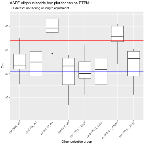
The above graph shows a visual summary of the Tm for the different ASPE-oligo’s. Another way to summarize the data is to do a basic table.
Table summary of the first attempt to generate ASPE-oligo’s
aspe_set %>%
    group_by(name) %>%
    summarize(n = n(),
              min_Tm = min(Tm),
              max_Tm = max(Tm),
              mean_Tm = mean(Tm),
              sd_Tm = sd(Tm)) %>%
    knitr::kable(caption = "Table summary of the different catagories of ASPE-oligo's")
Table: Table summary of the different catagories of ASPE-oligo’s
| name | n | min_Tm | max_Tm | mean_Tm | sd_Tm |
|---|---|---|---|---|---|
| canE69K_WT | 10 | 47.74501 | 57.51004 | 52.54260 | 2.863069 |
| canE76K_WT | 14 | 43.42922 | 59.09040 | 51.74416 | 4.719917 |
| canG503V_WT | 10 | 54.21869 | 62.05675 | 59.38974 | 2.556002 |
| canK91E_WT | 14 | 43.42922 | 53.96540 | 50.05479 | 3.843318 |
| canPTPN11_E69K | 10 | 45.58711 | 56.04576 | 50.77114 | 3.085982 |
| canPTPN11_E76K | 14 | 41.27132 | 57.80915 | 50.09424 | 4.995929 |
| canPTPN11_G503V | 10 | 52.06080 | 60.47983 | 57.61828 | 2.780629 |
| canPTPN11_K91E | 14 | 45.58711 | 55.24665 | 51.70471 | 3.570237 |
Adjusting ASPE oligo length of the entire data set.
After the summary for attempt one there are some regions that need the Tm changed. To do this the min and max oligo length need to be changed. Not all of the ASPE-Oligo’s need length change but the easiest way is to copy and paste the above code and then change min and max lengths.
aspe_set <- aspe_oligo(data = canPTPN11_E76K,
                           name = "canPTPN11_E76K",
                           point_mut = 393,
                           max_oligo_length = 34,
                           direction = "reverse",
                           Tm = TRUE) %>%
  rbind(., aspe_oligo(data = canPTPN11_WT,
                      name = "canE76K_WT",
                      point_mut = 393,
                      max_oligo_length = 31,
                      direction = "reverse",
                      Tm = TRUE)) %>%
  rbind(., aspe_oligo(data = canPTPN11_E69K,
                      name = "canPTPN11_E69K",
                      point_mut = 372,
                      max_oligo_length = 31,
                      Tm = TRUE)) %>%
  rbind(., aspe_oligo(data = canPTPN11_WT,
                      name = "canE69K_WT",
                      point_mut = 372,
                      max_oligo_length =  31,
                      Tm = TRUE)) %>%
  rbind(., aspe_oligo(data = canPTPN11_K91E,  ### Adjusting min and max
                      name = "canPTPN11_K91E",
                      point_mut = 438,
                      min_oligo_length = 18,
                      max_oligo_length = 34,
                      Tm = TRUE)) %>%
  rbind(., aspe_oligo(data = canPTPN11_WT,
                      name = "canK91E_WT",
                      point_mut = 438,
                      max_oligo_length = 35,
                      Tm = TRUE)) %>%
  rbind(., aspe_oligo(data = canPTPN11_G503V, ### Adjusted min and max
                      name = "canPTPN11_G503V",
                      point_mut = 1675,
                      min_oligo_length = 15,
                      max_oligo_length = 25,
                      Tm = TRUE)) %>%
  rbind(., aspe_oligo(data = canPTPN11_WT, ### adjusted min and max
                      name = "canG503V_WT",
                      point_mut = 1675,
                      min_oligo_length = 15,
                      max_oligo_length = 22,
                      Tm = TRUE))

### Going directly to the box/whisker plot
aspe_set %>%
    ggplot(., aes(x = name, y = Tm)) +
    geom_boxplot() +
    geom_hline(yintercept = 50.5, col = "Blue") +
    geom_hline(yintercept = 57, col = "Red") +
    theme(axis.text.x = element_text(angle = 45, hjust = 1)) +
    labs(title = "ASPE oligonucleotide box plot for Canine PTPN11 - Length Adjusted",
         x = "Oligonucleotide group",
         y = "Tm")
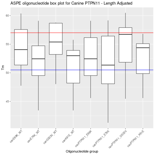
After graphing a generalized next step is to look at a summary table.
aspe_set %>%
    group_by(name) %>%
    summarize(n = n(),
              min_Tm = min(Tm),
              max_Tm = max(Tm),
              mean_Tm = mean(Tm),
              sd_Tm = sd(Tm)) %>%
  kable(caption = "Summary of the ASPE oligonucleotides in the aspe_set")
Table: Summary of the ASPE oligonucleotides in the aspe_set
| name | n | min_Tm | max_Tm | mean_Tm | sd_Tm |
|---|---|---|---|---|---|
| canE69K_WT | 14 | 47.74501 | 60.37165 | 54.39219 | 3.896502 |
| canE76K_WT | 14 | 43.42922 | 59.09040 | 51.74416 | 4.719917 |
| canG503V_WT | 8 | 48.02790 | 58.77247 | 54.99987 | 3.950733 |
| canK91E_WT | 18 | 43.42922 | 55.76401 | 51.14649 | 3.980133 |
| canPTPN11_E69K | 14 | 45.58711 | 59.09040 | 52.74227 | 4.168961 |
| canPTPN11_E76K | 17 | 41.27132 | 59.16004 | 51.61707 | 5.643207 |
| canPTPN11_G503V | 11 | 45.46540 | 60.47983 | 54.64570 | 4.680201 |
| canPTPN11_K91E | 17 | 45.58711 | 56.81719 | 52.44656 | 3.628126 |
Filtering the ASPE data frame by Tm
Filtering the data frame based upon Tm that is determined to be optimal for the Luminex mutli-plex ASPE assay.
filter_aspe_set <- aspe_set %>%
    filter(Tm >= 52 & Tm < 57) %>%
    slice_sample(., n = 25)

knitr::kable(filter_aspe_set, caption = "Random sample (n = 25)ASPE-oligo's with Tm >=52 and <57 deg C")
Table: Random sample (n = 25)ASPE-oligo’s with Tm >=52 and <57 deg C
| ASPE_oligo | dir | name | Tm |
|---|---|---|---|
| GCGGTCTCAGAGGTCAGG | forward | canG503V_WT | 53.90290 |
| ATTATATGGAACATCACGGACAATTAAAAGAGG | forward | canPTPN11_K91E | 55.38775 |
| TGGTGCGGTCTCAGAGGTCAGT | forward | canPTPN11_G503V | 56.85745 |
| GTGATGTTCCATATAATACTGGACCAACTT | reverse | canPTPN11_E76K | 54.93624 |
| GTGCGGTCTCAGAGGTCAGT | forward | canPTPN11_G503V | 54.50290 |
| ATATGGAACATCACGGACAATTAAAAGAGA | forward | canK91E_WT | 53.56957 |
| GAACATCACGGACAATTAAAAGAGG | forward | canPTPN11_K91E | 52.30290 |
| TTATATGGAACATCACGGACAATTAAAAGAGG | forward | canPTPN11_K91E | 55.24665 |
| TATATGGAACATCACGGACAATTAAAAGAGG | forward | canPTPN11_K91E | 55.09645 |
| ATGGAACATCACGGACAATTAAAAGAGA | forward | canK91E_WT | 53.11719 |
| GATGTTCCATATAATACTGGACCAACTT | reverse | canPTPN11_E76K | 53.11719 |
| GTATTATATGGAACATCACGGACAATTAAAAGAGG | forward | canPTPN11_K91E | 56.81719 |
| TATTATATGGAACATCACGGACAATTAAAAGAGA | forward | canK91E_WT | 54.31467 |
| GTGATTACTATGACTTGTATGGAGGGA | forward | canPTPN11_E69K | 54.38438 |
| TGTTCCATATAATACTGGACCAACTC | reverse | canE76K_WT | 52.59521 |
| CGTGATGTTCCATATAATACTGGACCAACTT | reverse | canPTPN11_E76K | 56.41903 |
| GTATTATATGGAACATCACGGACAATTAAAAGAGA | forward | canK91E_WT | 55.64576 |
| TGGAACATCACGGACAATTAAAAGAGA | forward | canK91E_WT | 52.86586 |
| TGGAACATCACGGACAATTAAAAGAGG | forward | canPTPN11_K91E | 54.38438 |
| TATGGAACATCACGGACAATTAAAAGAGG | forward | canPTPN11_K91E | 54.76497 |
| TGATGTTCCATATAATACTGGACCAACTC | reverse | canE76K_WT | 54.76497 |
| TGATTACTATGACTTGTATGGAGGGG | forward | canE69K_WT | 54.17213 |
| TGATGTTCCATATAATACTGGACCAACTT | reverse | canPTPN11_E76K | 53.35118 |
| TATTATATGGAACATCACGGACAATTAAAAGAGG | forward | canPTPN11_K91E | 55.52055 |
| ATGGTGCGGTCTCAGAGGTCAGT | forward | canPTPN11_G503V | 56.98986 |
Conclusion
This shows how R can be used to discover ASPE oligos, adjust length and filter based on Tm. The next step is to determine the downstream deterction method for the ASPE-oligo’s. If using a Bead Based Arrapy system a Luminex-MAGTAG bead specific complementary DNA sequence should be added. The addition of a magtag sequence will be shown in a later blog. The discovery/development of ASPE-oligos is a useful method to help rapidly screen for mutation that change the end base(s).
In future blogs, the use of online mutational databases (i.e. OMIM-ClinVar) and how to clean the data, extract the necessary information and generate ASPE oligo’s for detection will be demonstrated. Additionally, this data can be stored in a mariaDB table to make later retrieval easier for large mutational screening projects.
References
R Core Team (2022). R: A language and environment for statistical
computing. R Foundation for Statistical Computing, Vienna, Austria.
URL https://www.R-project.org/.
Wickham et al., (2019). Welcome to the tidyverse. Journal of Open
Source Software, 4(43), 1686, https://doi.org/10.21105/joss.01686
Li J (2022). TmCalculator: Melting Temperature of Nucleic Acid
Sequences. R package version 1.0.3,
https://CRAN.R-project.org/package=TmCalculator.
Olle E, W., (In Progress) The synxrna package: A tool for RNA
biomolecule generation and discovery. R pacakge in development